The Power of Simple Models: Why Complexity Isn't Always the Answer

Disclaimer: This article is not meant to diminish the incredible advancements being made with complex neural networks and AI models. As data science professionals, we deeply value and regularly implement sophisticated algorithms in appropriate contexts. The research community's work on advancing state-of-the-art AI is essential and transformative. This piece simply advocates for thoughtful model selection based on the specific problem at hand, recognizing that in some cases, simpler approaches may offer practical advantages.

In today's AI-driven landscape, there's a persistent narrative that more complex models yield better results. Social media, tech blogs, and YouTube tutorials bombard us with the same message:

"You should use Deep Learning™ & sophisticated Models" — Blogs, Reddit, Hacker News and YouTube Stars
‍

But as a data science leader with years of experience implementing both simple and complex solutions, I've come to appreciate an often-overlooked truth: the elegance and practical power of simpler models. While deep learning and complex algorithms have their place, the hype surrounding them often distracts us from understanding the actual problems we're trying to solve.

Understanding the Problem vs. Understanding the Solution

Vincent D. Warmerdam captured this perfectly when he said:

"When you understand the solution of the problem better than the problem itself, then something is wrong!"

This insight cuts to the heart of effective data science. Too often, we become experts at implementing complex algorithms without truly grasping the nuances of the problem at hand. We reach for sophisticated tools not because the problem demands it, but because it's what we know or what will impress our peers.

In my experience leading data science teams, I've observed a concerning trend: people focus more on the tools they're using than the problems they're solving. This isn't to say complex models aren't amazing—they absolutely are—but the hype around them can lead us astray from simple, elegant solutions.

The XOR Problem: A Perfect Example

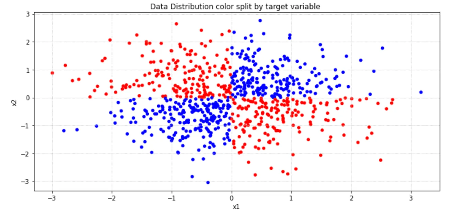
Let's look at a classic case that's used to dismiss linear models: the XOR problem.

Every machine learning textbook presents this as definitive proof that neural networks outperform standard regression. The argument is simple: linear models can only split data with a single line, while the XOR problem requires a non-linear solution because the dataset can't be separated by a single boundary.

This appears to be an open-and-shut case against linear models. But is it really?

A Simple Solution to a "Complex" Problem

When facing the XOR problem, our instinct is typically to reach for more complex algorithms—neural networks, SVMs with non-linear kernels, or other sophisticated approaches. These solutions work, but they come with drawbacks: reduced interpretability, implementation complexity, and potential maintenance headaches.

But what if we could solve the XOR problem with a simple linear model?

I ran an experiment demonstrating exactly this. Let's walk through the entire process, starting with creating our XOR dataset:

# Import necessary libraries
import pandas as pd
import numpy as np
import matplotlib.pyplot as plt
import patsy
from sklearn.linear_model import LogisticRegression
from sklearn.metrics import confusion_matrix, ConfusionMatrixDisplay, classification_report
from sklearn.svm import SVC

# Set a random seed for reproducibility
rng = np.random.RandomState(0)

# Create the XOR dataset with 750 samples
X_array = rng.randn(750, 2)  # Generate random data points
Y_array = np.logical_xor(X_array[:, 0] > 0, X_array[:, 1] > 0)  # Apply XOR logic

# Create a DataFrame for easier manipulation
X_df = pd.DataFrame(X_array, columns=['x1', 'x2'])
y_series = pd.Series(Y_array, name='type')
model_df = pd.concat([X_df, y_series], axis=1)
model_df.type = model_df.type.astype(int)

# Visualize the data
fig, ax = plt.subplots(figsize=(10, 5))
col = model_df.type.map({0:'b', 1:'r'})
model_df.plot.scatter(x='x1', y='x2', c=col, ax=ax,
                    title="Data Distribution color split by target variable")
plt.grid(linestyle=':')
plt.tight_layout()

‍

This creates our classic XOR pattern, where points in opposing quadrants share the same class. Looking at the plot, we can see the data isn't linearly separable with a single line.

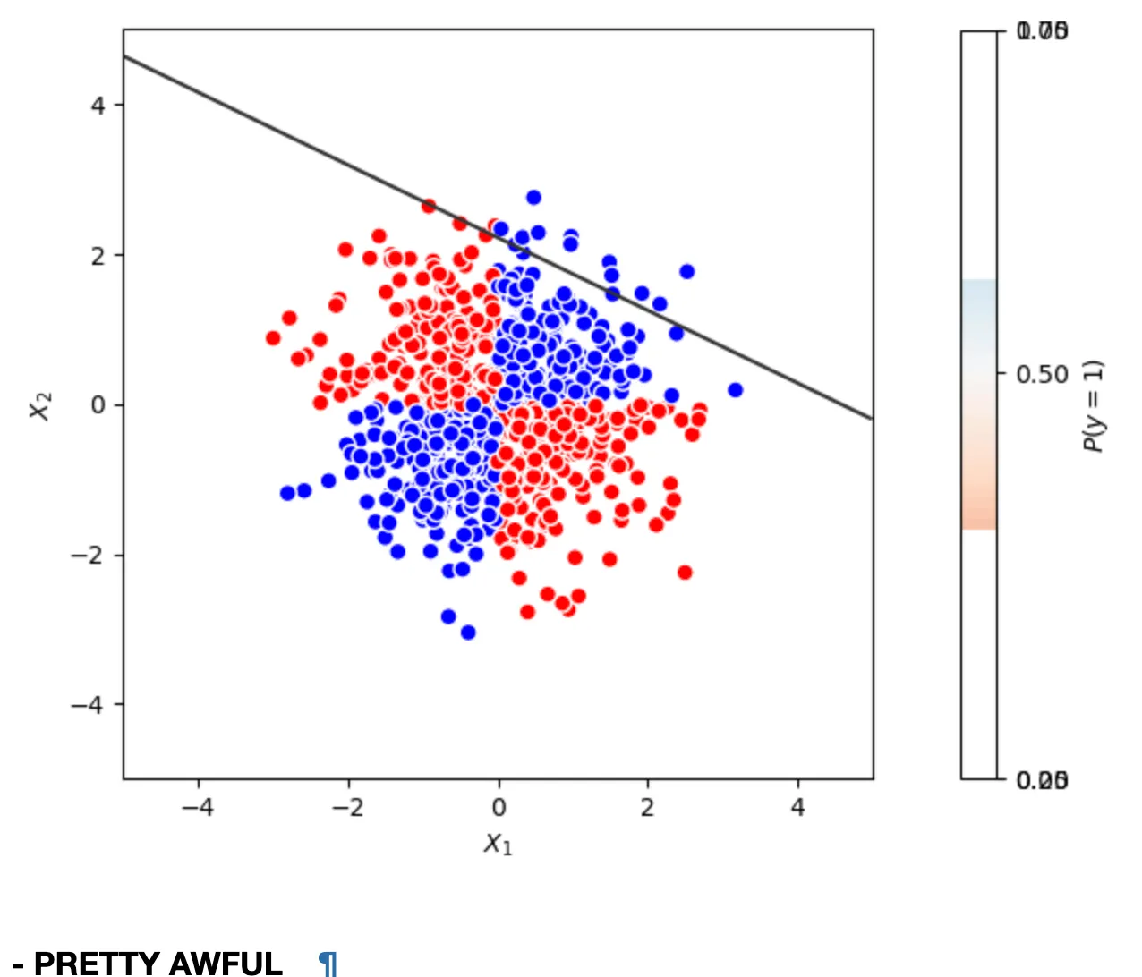
Next, I tried a standard logistic regression:

# Apply logistic regression to the XOR problem
y, X = patsy.dmatrices("type ~ x1 + x2", model_df)
pred = LogisticRegression().fit(X, y.reshape(-1, )).predict(X)
cm = confusion_matrix(y, pred)
cmd = ConfusionMatrixDisplay(cm, display_labels=['0','1'])
print(classification_report(y, pred))
cmd.plot()

# Visualize the decision boundary
X = model_df[['x1', 'x2']]
y = model_df.type
clf = LogisticRegression().fit(X, y)

# Create a grid to evaluate the model
xx, yy = np.mgrid[-5:5:.01, -5:5:.01]
grid = np.c_[xx.ravel(), yy.ravel()]
probs = clf.predict_proba(grid)[:, 1].reshape(xx.shape)

# Plot the decision boundary
f, ax = plt.subplots(figsize=(10, 4))
contour = ax.contourf(xx, yy, probs, 25, cmap="RdBu", vmin=0, vmax=1)
ax_c = f.colorbar(contour)
ax_c.set_label("$P(y = 1)$")
ax_c.set_ticks([0, .25, .5, .75, 1])

# Plot the data points
col = y.map({0:'b', 1:'r'})
X.plot.scatter(x='x1', y='x2', ax=ax, c=col, s=50, cmap="RdBu",
             vmin=-.2, vmax=1.2, edgecolor="white", linewidth=1,
             title="Decision Space")
ax.set(aspect="equal", xlim=(-5, 5), ylim=(-5, 5),
     xlabel="$X_1$", ylabel="$X_2$")
plt.tight_layout()

As expected, the model performed poorly, achieving only about 52% accuracy—barely better than random guessing. The decision boundary is simply a straight line, which can't capture the XOR pattern.

I then tried an SVM, which performed admirably:

# Try Support Vector Machine with default parameters
y, X = patsy.dmatrices("type ~ x1 + x2", model_df)
pred = SVC(probability=True).fit(X, y.reshape(-1, )).predict(X)
cm = confusion_matrix(y, pred)
cmd = ConfusionMatrixDisplay(cm, display_labels=['0','1'])
print(classification_report(y, pred))
cmd.plot()

# Visualize the SVM decision boundary
X = model_df[['x1', 'x2']]
y = model_df.type
clf = SVC(probability=True).fit(X, y)

# Create a grid to evaluate the model
xx, yy = np.mgrid[-5:5:.01, -5:5:.01]
grid = np.c_[xx.ravel(), yy.ravel()]
probs = clf.predict_proba(grid)[:, 1].reshape(xx.shape)

# Plot the decision boundary
f, ax = plt.subplots(figsize=(10, 5))
contour = ax.contourf(xx, yy, probs, 25, cmap="RdBu", vmin=0, vmax=1)
ax_c = f.colorbar(contour)
ax_c.set_label("$P(y = 1)$")
ax_c.set_ticks([0, .25, .5, .75, 1])

# Plot the data points
col = y.map({0:'b', 1:'r'})
X.plot.scatter(x='x1', y='x2', ax=ax, c=col, s=50, cmap="RdBu",
             vmin=-.2, vmax=1.2, edgecolor="white", linewidth=1)
ax.set(aspect="equal", xlim=(-5, 5), ylim=(-5, 5),
     xlabel="$X_1$", ylabel="$X_2$")
plt.tight_layout()

The SVM achieved around 95% accuracy with a beautiful non-linear decision boundary that perfectly captured the XOR pattern. Success! But at what cost?

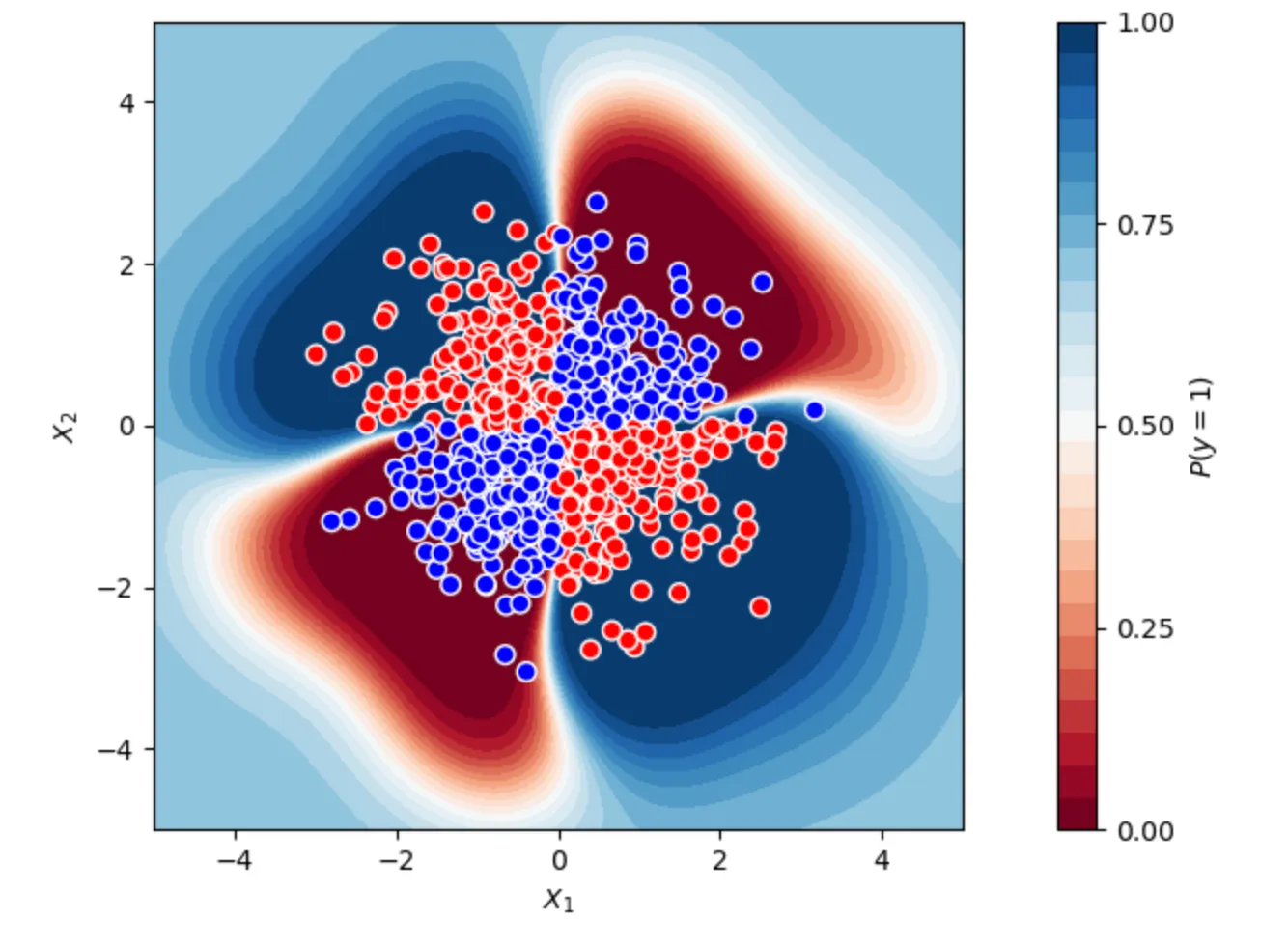
The SVM solution, while effective, is a black box. If it fails in production, diagnosing the issue would be challenging. Do we really need this complexity?

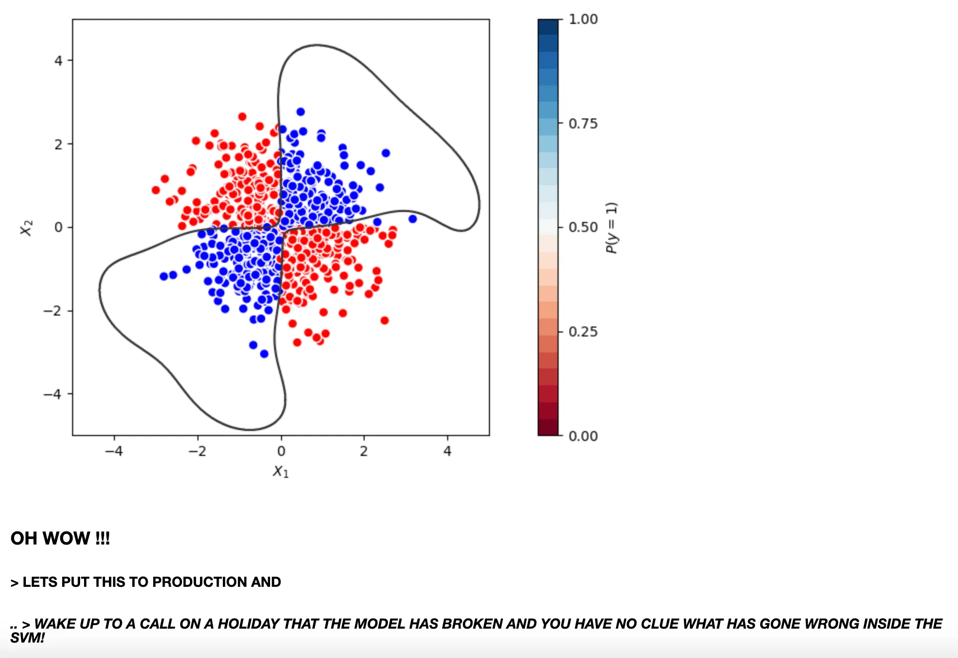
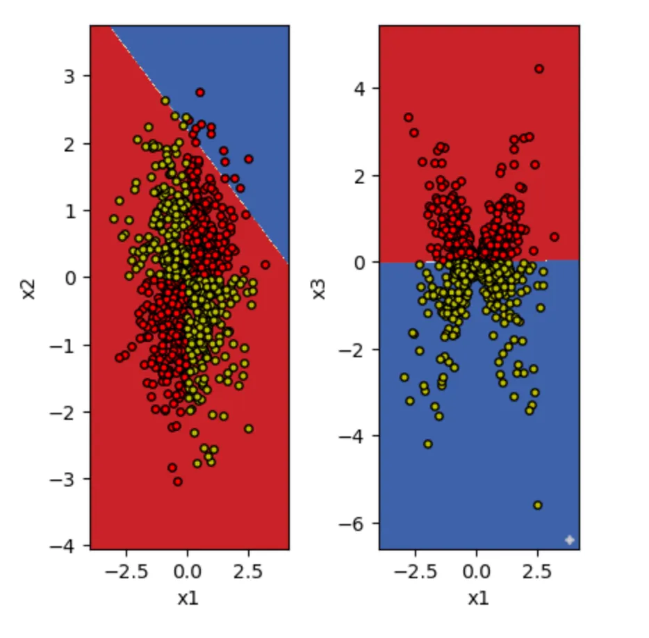
Here's where feature engineering shines. By adding just one new feature—the product of our existing features—we can transform the problem:

‍

# Create a new feature: the interaction term x1*x2
model_df['x3'] = model_df['x1'] * model_df['x2']

# Apply logistic regression with the new feature
y, X = patsy.dmatrices("type ~ x1 + x2 + x3", model_df)
pred = LogisticRegression().fit(X, y.reshape(-1, )).predict(X)
cm = confusion_matrix(y, pred)
cmd = ConfusionMatrixDisplay(cm, display_labels=['0','1'])
print(classification_report(y, pred))
cmd.plot()

# Visualize the decision space with our new feature
X_df = model_df[['x1', 'x2', 'x3']]
y_df = model_df.type

# Parameters for plotting
n_classes = 2
plot_colors = "ryb"
plot_step = 0.02

# Plot decision boundaries for different feature pairs
for pairidx, pair in enumerate([[0, 1], [0, 2]]):
   # Take two corresponding features
   X = X_df.values[:, pair]
   y = y_df

   # Train
   clf = LogisticRegression().fit(X, y)

   # Plot the decision boundary
   plt.subplot(1, 3, pairidx + 1)
   x_min, x_max = X[:, 0].min() - 1, X[:, 0].max() + 1
   y_min, y_max = X[:, 1].min() - 1, X[:, 1].max() + 1
   xx, yy = np.meshgrid(np.arange(x_min, x_max, plot_step),
                        np.arange(y_min, y_max, plot_step))
   plt.tight_layout(h_pad=0.5, w_pad=0.5, pad=2.5)

   Z = clf.predict(np.c_[xx.ravel(), yy.ravel()])
   Z = Z.reshape(xx.shape)
   cs = plt.contourf(xx, yy, Z, cmap=plt.cm.RdYlBu)

   plt.xlabel(X_df.columns[pair[0]])
   plt.ylabel(X_df.columns[pair[1]])

   # Plot the training points
   for i, color in zip(range(n_classes), plot_colors):
       idx = np.where(y == i)
       plt.scatter(X[idx, 0], X[idx, 1], c=color, cmap=plt.cm.RdYlBu,
                  edgecolor='black', s=15)

plt.suptitle("Decision surface using paired features")
plt.axis("tight")
plt.tight_layout()

The result? An impressive 98% accuracy—even better than the SVM—while maintaining the interpretability and simplicity of a linear model. With just one additional feature, our linear model can now create a curved decision boundary that perfectly captures the XOR pattern.

Why This Matters Beyond the Notebook

This isn't just an academic exercise. In production environments, model properties beyond raw accuracy become critical:

1. Interpretability: Stakeholders can understand what drives predictions
2. Maintainability: Team members can understand and update the model
3. Stability: The model behaves predictably when deployed
4. Fewer production failures: Simpler models have fewer points of failure

As a consultant, I've found it's much easier to leave clients with a well-engineered linear model—especially if they're just beginning their modeling journey—than a complex black-box solution that might require specialized knowledge to maintain.

When to Embrace Simplicity

Of course, this doesn't mean we should never use complex models. Deep learning has revolutionized many domains for good reason. The key is to add complexity thoughtfully, only when:

1. You've established that simpler approaches don't meet your requirements
2. You understand why the additional complexity is necessary
3. The performance improvement justifies the trade-offs
4. You've considered the full lifecycle of the model

A Call to Problem-Centric Thinking

The next time you approach a data problem, resist the immediate urge to reach for the latest algorithm. Instead:

1. Define the problem clearly: What are you really trying to solve?
2. Start simple: Can feature engineering with a linear model get you most of the way there?
3. Measure what matters: Does improved accuracy on a test set translate to real-world value?
4. Add complexity incrementally: Can you justify each layer of sophistication?

‍

And the next time someone says, "Oh, you've created a linear regression to solve this?" remember that your choice reflects wisdom, not limitation. You've focused on the problem rather than the solution—and that's something to be proud of.

Conclusion

It's not that deep learning and complex models aren't valuable—they absolutely are. But the hype around them can distract us from great ideas and simpler solutions that might be more appropriate for our specific problems.

As data scientists, our job isn't to implement algorithms—it's to solve problems. Sometimes, that means having the courage to embrace simplicity in a field that often rewards complexity.

So let's explore the domain of "boring, old but ultimately beautiful simple models" with fresh eyes. With thoughtful feature engineering and a solid understanding of our problems, we might find that the simplest solution is often the most elegant and effective one.

‍

This blog was inspired by Vincent Warmerdam's PyData London 2018 talk "Winning with Simple, even Linear, Models" and my own experiences implementing these principles in production environments.